Sorting algorithm

History

From the beginning of computing, the sorting problem has attracted a great deal of research, perhaps due to the complexity of solving it efficiently despite its simple, familiar statement. Among the authors of early sorting algorithms around 1951 was Betty Holberton (born Snyder), who worked on ENIAC and UNIVAC.^[1][2]Bubble sort was analyzed as early as 1956.^[3] Comparison sorting algorithms have a fundamental requirement of Ω(n log n) comparisons (some input sequences will require a multiple of n log n comparisons, where n is the number of elements in the array to be sorted). Algorithms not based on comparisons, such as counting sort, can have better performance. Asymptotically optimal algorithms have been known since the mid-20th century—useful new algorithms are still being invented, with the now widely used Timsort dating to 2002, and the library sort being first published in 2006.

Sorting algorithms are prevalent in introductory computer science classes, where the abundance of algorithms for the problem provides a gentle introduction to a variety of core algorithm concepts, such as big O notation, divide and conquer algorithms, data structures such as heaps and binary trees, randomized algorithms, best, worst and average case analysis, time–space tradeoffs, and upper and lower bounds.

Sorting small arrays optimally (in least amount of comparisons and swaps) or fast (i.e. taking into account machine specific details) is still an open research problem, with solutions only known for very small arrays (<20 elements). Similarly optimal (by various definition) sorting on a parallel machine is an open research topic.

Classification

Sorting algorithms are often classified by:

• Computational complexity (worst, average and best behavior) in terms of the size of the list (n). For typical serial sorting algorithms good behavior is O(n log n), with parallel sort in O(log² n), and bad behavior is O(n²). (See Big O notation.) Ideal behavior for a serial sort is O(n), but this is not possible in the average case. Optimal parallel sorting is O(log n). Comparison-based sorting algorithms need at least Ω(n log n) comparisons for most inputs.
• Computational complexity of swaps (for "in-place" algorithms).
• Memory usage (and use of other computer resources). In particular, some sorting algorithms are "in-place". Strictly, an in-place sort needs only O(1) memory beyond the items being sorted; sometimes O(log(n)) additional memory is considered "in-place".
• Recursion. Some algorithms are either recursive or non-recursive, while others may be both (e.g., merge sort).
• Stability: stable sorting algorithms maintain the relative order of records with equal keys (i.e., values).
• Whether or not they are a comparison sort. A comparison sort examines the data only by comparing two elements with a comparison operator.
• General method: insertion, exchange, selection, merging, etc. Exchange sorts include bubble sort and quicksort. Selection sorts include shaker sort and heapsort.
• Whether the algorithm is serial or parallel. The remainder of this discussion almost exclusively concentrates upon serial algorithms and assumes serial operation.
• Adaptability: Whether or not the presortedness of the input affects the running time. Algorithms that take this into account are known to be adaptive.
• Online: An algorithm such as Insertion Sort that is online can sort a constant stream of input.

Stability

An example of stable sort on playing cards. When the cards are sorted by rank with a stable sort, the two 5s must remain in the same order in the sorted output that they were originally in. When they are sorted with a non-stable sort, the 5s may end up in the opposite order in the sorted output.

Stable sort algorithms sort repeated elements in the same order that they appear in the input. When sorting some kinds of data, only part of the data is examined when determining the sort order. For example, in the card sorting example to the right, the cards are being sorted by their rank, and their suit is being ignored. This allows the possibility of multiple different correctly sorted versions of the original list. Stable sorting algorithms choose one of these, according to the following rule: if two items compare as equal, like the two 5 cards, then their relative order will be preserved, so that if one came before the other in the input, it will also come before the other in the output.

Stability is important for the following reason: say that student records consisting of name and class section are sorted dynamically on a web page, first by name, then by class section in a second operation. If a stable sorting algorithm is used in both cases, the sort-by-class-section operation will not change the name order; with an unstable sort, it could be that sorting by section shuffles the name order. Using a stable sort, users can choose to sort by section and then by name, by first sorting using name and then sort again using section, resulting in the name order being preserved. (Some spreadsheet programs obey this behavior: sorting by name, then by section yields an alphabetical list of students by section.)
Another reason: unstable sort may yield different output for the same input from run to run. Such behavior is unsuitable for some applications, for example for client-server applications where the server uses pagination for output and performs a new search-and-sort for every new page requested by the client.

More formally, the data being sorted can be represented as a record or tuple of values, and the part of the data that is used for sorting is called the key. In the card example, cards are represented as a record (rank, suit), and the key is the rank. A sorting algorithm is stable if whenever there are two records R and S with the same key, and R appears before S in the original list, then R will always appear before S in the sorted list.

When equal elements are indistinguishable, such as with integers, or more generally, any data where the entire element is the key, stability is not an issue. Stability is also not an issue if all keys are different.

Unstable sorting algorithms can be specially implemented to be stable. One way of doing this is to artificially extend the key comparison, so that comparisons between two objects with otherwise equal keys are decided using the order of the entries in the original input list as a tie-breaker. Remembering this order, however, may require additional time and space.

One application for stable sorting algorithms is sorting a list using a primary and secondary key. For example, suppose we wish to sort a hand of cards such that the suits are in the order clubs (♣), diamonds (♦), hearts (♥), spades (♠), and within each suit, the cards are sorted by rank. This can be done by first sorting the cards by rank (using any sort), and then doing a stable sort by suit:

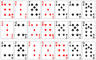
Within each suit, the stable sort preserves the ordering by rank that was already done. This idea can be extended to any number of keys and is utilised by radix sort. The same effect can be achieved with an unstable sort by using a lexicographic key comparison, which, e.g., compares first by suit, and then compares by rank if the suits are the same.

Comparison of algorithms

In this table, n is the number of records to be sorted. The columns "Average" and "Worst" give the time complexity in each case, under the assumption that the length of each key is constant, and that therefore all comparisons, swaps, and other needed operations can proceed in constant time. "Memory" denotes the amount of auxiliary storage needed beyond that used by the list itself, under the same assumption. The run times and the memory requirements listed below should be understood to be inside big O notation, hence the base of the logarithms does not matter; the notation log²n means (log n)².

Comparison sorts

Below is a table of comparison sorts. A comparison sort cannot perform better than O(n log n) on average.^[4]

Comparison sorts

Name	Best	Average	Worst	Memory	Stable	Method	Other notes
Quicksort	${\displaystyle n\log n}$	${\displaystyle n\log n}$	${\displaystyle n^{2}}$	${\displaystyle \log n}$	No	Partitioning	Quicksort is usually done in-place with O(log n) stack space.[5][6]
Merge sort	${\displaystyle n\log n}$	${\displaystyle n\log n}$	${\displaystyle n\log n}$	n	Yes	Merging	Highly parallelizable (up to O(log n) using the Three Hungarians' Algorithm).[7]
In-place merge sort	—	—	${\displaystyle n\log ^{2}n}$	1	Yes	Merging	Can be implemented as a stable sort based on stable in-place merging.[8]
Introsort	${\displaystyle n\log n}$	${\displaystyle n\log n}$	${\displaystyle n\log n}$	${\displaystyle \log n}$	No	Partitioning & Selection	Used in several STL implementations.
Heapsort	${\displaystyle n\log n}$	${\displaystyle n\log n}$	${\displaystyle n\log n}$	1	No	Selection
Insertion sort	n	${\displaystyle n^{2}}$	${\displaystyle n^{2}}$	1	Yes	Insertion	O(n + d), in the worst case over sequences that have d inversions.
Block sort	n	${\displaystyle n\log n}$	${\displaystyle n\log n}$	1	Yes	Insertion & Merging	Combine a block-based ${\displaystyle O(n)}$ in-place merge algorithm[9] with a bottom-up merge sort.
Quadsort	n	${\displaystyle n\log n}$	${\displaystyle n\log n}$	n	Yes	Merging	Uses a 4-input sorting network.[10]
Timsort	n	${\displaystyle n\log n}$	${\displaystyle n\log n}$	n	Yes	Insertion & Merging	Makes n comparisons when the data is already sorted or reverse sorted.
Selection sort	${\displaystyle n^{2}}$	${\displaystyle n^{2}}$	${\displaystyle n^{2}}$	1	No	Selection	Stable with ${\displaystyle O(n)}$ extra space or when using linked lists.[11]
Cubesort	n	${\displaystyle n\log n}$	${\displaystyle n\log n}$	n	Yes	Insertion	Makes n comparisons when the data is already sorted or reverse sorted.
Shellsort	${\displaystyle n\log n}$	${\displaystyle n^{4/3}}$	${\displaystyle n^{3/2}}$	1	No	Insertion	Small code size.
Bubble sort	n	${\displaystyle n^{2}}$	${\displaystyle n^{2}}$	1	Yes	Exchanging	Tiny code size.
Tree sort	${\displaystyle n\log n}$	${\displaystyle n\log n}$	${\displaystyle n\log n}$(balanced)	n	Yes	Insertion	When using a self-balancing binary search tree.
Cycle sort	${\displaystyle n^{2}}$	${\displaystyle n^{2}}$	${\displaystyle n^{2}}$	1	No	Selection	In-place with theoretically optimal number of writes.
Library sort	${\displaystyle n\log n}$	${\displaystyle n\log n}$	${\displaystyle n^{2}}$	n	No	Insertion	Similar to a gapped insertion sort. It requires randomly permuting the input to warrant with-high-probability time bounds, which makes it not stable.
Patience sorting	n	${\displaystyle n\log n}$	${\displaystyle n\log n}$	n	No	Insertion & Selection	Finds all the longest increasing subsequences in O(n log n).
Smoothsort	n	${\displaystyle n\log n}$	${\displaystyle n\log n}$	1	No	Selection	An adaptive variant of heapsort based upon the Leonardo sequence rather than a traditional binary heap.
Strand sort	n	${\displaystyle n^{2}}$	${\displaystyle n^{2}}$	n	Yes	Selection
Tournament sort	${\displaystyle n\log n}$	${\displaystyle n\log n}$	${\displaystyle n\log n}$	n[12]	No	Selection	Variation of Heap Sort.
Cocktail shaker sort	n	${\displaystyle n^{2}}$	${\displaystyle n^{2}}$	1	Yes	Exchanging	A variant of Bubblesort which deals well with small values at end of list
Comb sort	${\displaystyle n\log n}$	${\displaystyle n^{2}}$	${\displaystyle n^{2}}$	1	No	Exchanging	Faster than bubble sort on average.
Gnome sort	n	${\displaystyle n^{2}}$	${\displaystyle n^{2}}$	1	Yes	Exchanging	Tiny code size.
UnShuffle Sort[13]	n	kn	kn	n	No	Distribution and Merge	No exchanges are performed. The parameter k is proportional to the entropy in the input. k = 1 for ordered or reverse ordered input.
Franceschini's method[14]	n	${\displaystyle n\log n}$	${\displaystyle n\log n}$	1	Yes	?	Performs O(n) data moves.
Odd–even sort	n	${\displaystyle n^{2}}$	${\displaystyle n^{2}}$	1	Yes	Exchanging	Can be run on parallel processors easily.

Non-comparison sorts

The following table describes integer sorting algorithms and other sorting algorithms that are not comparison sorts. As such, they are not limited to Ω(n log n).^[15] Complexities below assume n items to be sorted, with keys of size k, digit size d, and r the range of numbers to be sorted. Many of them are based on the assumption that the key size is large enough that all entries have unique key values, and hence that n ≪ 2^k, where ≪ means "much less than". In the unit-cost random-access machine model, algorithms with running time of ${\displaystyle \scriptstyle n\cdot {\frac {k}{d}}}$, such as radix sort, still take time proportional to Θ(n log n), because n is limited to be not more than ${\displaystyle 2^{\frac {k}{d}}}$, and a larger number of elements to sort would require a bigger k in order to store them in the memory.^[16]

Non-comparison sorts

Name	Best	Average	Worst	Memory	Stable	n ≪ 2k	Notes
Pigeonhole sort	—	${\displaystyle n+2^{k}}$	${\displaystyle n+2^{k}}$	${\displaystyle 2^{k}}$	Yes	Yes	Cannot sort non-integers.
Bucket sort (uniform keys)	—	${\displaystyle n+k}$	${\displaystyle n^{2}\cdot k}$	${\displaystyle n\cdot k}$	Yes	No	Assumes uniform distribution of elements from the domain in the array. [17] Also cannot sort non-integers
Bucket sort (integer keys)	—	${\displaystyle n+r}$	${\displaystyle n+r}$	${\displaystyle n+r}$	Yes	Yes	If r is ${\displaystyle O(n)}$, then average time complexity is ${\displaystyle O(n)}$.[18]
Counting sort	—	${\displaystyle n+r}$	${\displaystyle n+r}$	${\displaystyle n+r}$	Yes	Yes	If r is ${\displaystyle O(n)}$, then average time complexity is ${\displaystyle O(n)}$.[17]
LSD Radix Sort	${\displaystyle n}$	${\displaystyle n\cdot {\frac {k}{d}}}$	${\displaystyle n\cdot {\frac {k}{d}}}$	${\displaystyle n+2^{d}}$	Yes	No	${\displaystyle {\frac {k}{d}}}$ recursion levels, 2d for count array.[17][18] Unlike most distribution sorts, this can sort Floating point numbers, negative numbers and more.
MSD Radix Sort	—	${\displaystyle n\cdot {\frac {k}{d}}}$	${\displaystyle n\cdot {\frac {k}{d}}}$	${\displaystyle n+2^{d}}$	Yes	No	Stable version uses an external array of size n to hold all of the bins. Same as the LSD variant, it can sort non-integers.
MSD Radix Sort (in-place)	—	${\displaystyle n\cdot {\frac {k}{1}}}$	${\displaystyle n\cdot {\frac {k}{1}}}$	${\displaystyle 2^{1}}$	No	No	d=1 for in-place, ${\displaystyle k/1}$ recursion levels, no count array.
Spreadsort	n	${\displaystyle n\cdot {\frac {k}{d}}}$	${\displaystyle n\cdot \left({{\frac {k}{s}}+d}\right)}$	${\displaystyle {\frac {k}{d}}\cdot 2^{d}}$	No	No	Asymptotic are based on the assumption that n ≪ 2k, but the algorithm does not require this.
Burstsort	—	${\displaystyle n\cdot {\frac {k}{d}}}$	${\displaystyle n\cdot {\frac {k}{d}}}$	${\displaystyle n\cdot {\frac {k}{d}}}$	No	No	Has better constant factor than radix sort for sorting strings. Though relies somewhat on specifics of commonly encountered strings.
Flashsort	n	${\displaystyle n+r}$	${\displaystyle n^{2}}$	n	No	No	Requires uniform distribution of elements from the domain in the array to run in linear time. If distribution is extremely skewed then it can go quadratic if underlying sort is quadratic (it is usually an insertion sort). In-place version is not stable.
Postman sort	—	${\displaystyle n\cdot {\frac {k}{d}}}$	${\displaystyle n\cdot {\frac {k}{d}}}$	${\displaystyle n+2^{d}}$	—	No	A variation of bucket sort, which works very similar to MSD Radix Sort. Specific to post service needs.
Sleep Sort[19]	—	—	—	—	—	—	For each item, a separate task is created that sleeps for an interval corresponding to the item's sort key. The items are then emitted and collected sequentially in time.

Samplesort can be used to parallelize any of the non-comparison sorts, by efficiently distributing data into several buckets and then passing down sorting to several processors, with no need to merge as buckets are already sorted between each other.

Others

Some algorithms are slow compared to those discussed above, such as the bogosort with unbounded run time and the stooge sort which has O(n^2.7) run time. These sorts are usually described for educational purposes in order to demonstrate how run time of algorithms is estimated. The following table describes some sorting algorithms that are impractical for real-life use in traditional software contexts due to extremely poor performance or specialized hardware requirements.

Name	Best	Average	Worst	Memory	Stable	Comparison	Other notes
Bead sort	n	S	S	${\displaystyle n^{2}}$	N/A	No	Works only with positive integers. Requires specialized hardware for it to run in guaranteed ${\displaystyle O(n)}$ time. There is a possibility for software implementation, but running time will be ${\displaystyle O(S)}$, where S is sum of all integers to be sorted, in case of small integers it can be considered to be linear.
Simple pancake sort	—	n	n	${\displaystyle \log n}$	No	Yes	Count is number of flips.
Spaghetti (Poll) sort	n	n	n	${\displaystyle n^{2}}$	Yes	Polling	This is a linear-time, analog algorithm for sorting a sequence of items, requiring O(n) stack space, and the sort is stable. This requires n parallel processors. See spaghetti sort#Analysis.
Sorting network	${\displaystyle \log ^{2}n}$	${\displaystyle \log ^{2}n}$	${\displaystyle \log ^{2}n}$	${\displaystyle n\log ^{2}n}$	Varies (stable sorting networks require more comparisons)	Yes	Order of comparisons are set in advance based on a fixed network size. Impractical for more than 32 items.[disputed – discuss]
Bitonic sorter	${\displaystyle \log ^{2}n}$	${\displaystyle \log ^{2}n}$	${\displaystyle \log ^{2}n}$	${\displaystyle n\log ^{2}n}$	No	Yes	An effective variation of Sorting networks.
Bogosort	n	${\displaystyle (n\times n!)}$	unbounded (certain), ${\displaystyle (n\times n!)}$ (expected)	1	No	Yes	Random shuffling. Used for example purposes only, as even the expected best-case runtime is awful.[20]
Stooge sort	${\displaystyle n^{\log 3/\log 1.5}}$	${\displaystyle n^{\log 3/\log 1.5}}$	${\displaystyle n^{\log 3/\log 1.5}}$	n	No	Yes	Slower than most of the sorting algorithms (even naive ones) with a time complexity of O(nlog 3 / log 1.5 ) = O(n2.7095...).

Theoretical computer scientists have detailed other sorting algorithms that provide better than O(n log n) time complexity assuming additional constraints, including:

• Thorup's algorithm, a randomized algorithm for sorting keys from a domain of finite size, taking O(n log log n) time and O(n) space.^[21]
• A randomized integer sorting algorithm taking ${\displaystyle O\left(n{\sqrt {\log \log n}}\right)}$ expected time and O(n) space.^[22]

Popular sorting algorithms

While there are a large number of sorting algorithms, in practical implementations a few algorithms predominate. Insertion sort is widely used for small data sets, while for large data sets an asymptotically efficient sort is used, primarily heap sort, merge sort, or quicksort. Efficient implementations generally use a hybrid algorithm, combining an asymptotically efficient algorithm for the overall sort with insertion sort for small lists at the bottom of a recursion. Highly tuned implementations use more sophisticated variants, such as Timsort (merge sort, insertion sort, and additional logic), used in Android, Java, and Python, and introsort (quicksort and heap sort), used (in variant forms) in some C++ sort implementations and in .NET.

For more restricted data, such as numbers in a fixed interval, distribution sorts such as counting sort or radix sort are widely used. Bubble sort and variants are rarely used in practice, but are commonly found in teaching and theoretical discussions.

When physically sorting objects (such as alphabetizing papers, tests or books) people intuitively generally use insertion sorts for small sets. For larger sets, people often first bucket, such as by initial letter, and multiple bucketing allows practical sorting of very large sets. Often space is relatively cheap, such as by spreading objects out on the floor or over a large area, but operations are expensive, particularly moving an object a large distance – locality of reference is important. Merge sorts are also practical for physical objects, particularly as two hands can be used, one for each list to merge, while other algorithms, such as heap sort or quick sort, are poorly suited for human use. Other algorithms, such as library sort, a variant of insertion sort that leaves spaces, are also practical for physical use.

Simple sorts

Two of the simplest sorts are insertion sort and selection sort, both of which are efficient on small data, due to low overhead, but not efficient on large data. Insertion sort is generally faster than selection sort in practice, due to fewer comparisons and good performance on almost-sorted data, and thus is preferred in practice, but selection sort uses fewer writes, and thus is used when write performance is a limiting factor.

Insertion sort

Insertion sort is a simple sorting algorithm that is relatively efficient for small lists and mostly sorted lists, and is often used as part of more sophisticated algorithms. It works by taking elements from the list one by one and inserting them in their correct position into a new sorted list similar to how we put money in our wallet.^[23] In arrays, the new list and the remaining elements can share the array's space, but insertion is expensive, requiring shifting all following elements over by one. Shellsort (see below) is a variant of insertion sort that is more efficient for larger lists.

Selection sort

Selection sort is an in-place comparison sort. It has O(n²) complexity, making it inefficient on large lists, and generally performs worse than the similar insertion sort. Selection sort is noted for its simplicity, and also has performance advantages over more complicated algorithms in certain situations.

The algorithm finds the minimum value, swaps it with the value in the first position, and repeats these steps for the remainder of the list.^[24] It does no more than n swaps, and thus is useful where swapping is very expensive.

Efficient sorts

Practical general sorting algorithms are almost always based on an algorithm with average time complexity (and generally worst-case complexity) O(n log n), of which the most common are heap sort, merge sort, and quicksort. Each has advantages and drawbacks, with the most significant being that simple implementation of merge sort uses O(n) additional space, and simple implementation of quicksort has O(n²) worst-case complexity. These problems can be solved or ameliorated at the cost of a more complex algorithm.

While these algorithms are asymptotically efficient on random data, for practical efficiency on real-world data various modifications are used. First, the overhead of these algorithms becomes significant on smaller data, so often a hybrid algorithm is used, commonly switching to insertion sort once the data is small enough. Second, the algorithms often perform poorly on already sorted data or almost sorted data – these are common in real-world data, and can be sorted in O(n) time by appropriate algorithms. Finally, they may also be unstable, and stability is often a desirable property in a sort. Thus more sophisticated algorithms are often employed, such as Timsort (based on merge sort) or introsort (based on quicksort, falling back to heap sort).

Merge sort

Merge sort takes advantage of the ease of merging already sorted lists into a new sorted list. It starts by comparing every two elements (i.e., 1 with 2, then 3 with 4...) and swapping them if the first should come after the second. It then merges each of the resulting lists of two into lists of four, then merges those lists of four, and so on; until at last two lists are merged into the final sorted list.^[25] Of the algorithms described here, this is the first that scales well to very large lists, because its worst-case running time is O(n log n). It is also easily applied to lists, not only arrays, as it only requires sequential access, not random access. However, it has additional O(n) space complexity, and involves a large number of copies in simple implementations.

Merge sort has seen a relatively recent surge in popularity for practical implementations, due to its use in the sophisticated algorithm Timsort, which is used for the standard sort routine in the programming languages Python^[26] and Java (as of JDK7^[27]). Merge sort itself is the standard routine in Perl,^[28] among others, and has been used in Java at least since 2000 in JDK1.3.^[29]

Heapsort

Heapsort is a much more efficient version of selection sort. It also works by determining the largest (or smallest) element of the list, placing that at the end (or beginning) of the list, then continuing with the rest of the list, but accomplishes this task efficiently by using a data structure called a heap, a special type of binary tree.^[30] Once the data list has been made into a heap, the root node is guaranteed to be the largest (or smallest) element. When it is removed and placed at the end of the list, the heap is rearranged so the largest element remaining moves to the root. Using the heap, finding the next largest element takes O(log n) time, instead of O(n) for a linear scan as in simple selection sort. This allows Heapsort to run in O(n log n) time, and this is also the worst case complexity.

Quicksort

Quicksort is a divide and conquer algorithm which relies on a partition operation: to partition an array, an element called a pivot is selected.^[31][32] All elements smaller than the pivot are moved before it and all greater elements are moved after it. This can be done efficiently in linear time and in-place. The lesser and greater sublists are then recursively sorted. This yields average time complexity of O(n log n), with low overhead, and thus this is a popular algorithm. Efficient implementations of quicksort (with in-place partitioning) are typically unstable sorts and somewhat complex, but are among the fastest sorting algorithms in practice. Together with its modest O(log n) space usage, quicksort is one of the most popular sorting algorithms and is available in many standard programming libraries.

The important caveat about quicksort is that its worst-case performance is O(n²); while this is rare, in naive implementations (choosing the first or last element as pivot) this occurs for sorted data, which is a common case. The most complex issue in quicksort is thus choosing a good pivot element, as consistently poor choices of pivots can result in drastically slower O(n²) performance, but good choice of pivots yields O(n log n) performance, which is asymptotically optimal. For example, if at each step the median is chosen as the pivot then the algorithm works in O(n log n). Finding the median, such as by the median of medians selection algorithm is however an O(n) operation on unsorted lists and therefore exacts significant overhead with sorting. In practice choosing a random pivot almost certainly yields O(n log n) performance.

Shellsort

A Shell sort, different from bubble sort in that it moves elements to numerous swapping positions.

Shellsort was invented by Donald Shell in 1959.^[33] It improves upon insertion sort by moving out of order elements more than one position at a time. The concept behind Shellsort is that insertion sort performs in ${\displaystyle O(kn)}$ time, where k is the greatest distance between two out-of-place elements. This means that generally, they perform in O(n²), but for data that is mostly sorted, with only a few elements out of place, they perform faster. So, by first sorting elements far away, and progressively shrinking the gap between the elements to sort, the final sort computes much faster. One implementation can be described as arranging the data sequence in a two-dimensional array and then sorting the columns of the array using insertion sort.

The worst-case time complexity of Shellsort is an open problem and depends on the gap sequence used, with known complexities ranging from O(n²) to O(n^4/3) and Θ(n log²n). This, combined with the fact that Shellsort is in-place, only needs a relatively small amount of code, and does not require use of the call stack, makes it is useful in situations where memory is at a premium, such as in embedded systems and operating system kernels.

Bubble sort and variants

This section does not cite any sources. Please help improve this section by adding citations to reliable sources. Unsourced material may be challenged and removed. (May 2019) (Learn how and when to remove this template message)

Bubble sort, and variants such as the shell sort and cocktail sort, are simple, highly inefficient sorting algorithms. They are frequently seen in introductory texts due to ease of analysis, but they are rarely used in practice.

Bubble sort

A bubble sort, a sorting algorithm that continuously steps through a list, swapping items until they appear in the correct order.

Bubble sort is a simple sorting algorithm. The algorithm starts at the beginning of the data set. It compares the first two elements, and if the first is greater than the second, it swaps them. It continues doing this for each pair of adjacent elements to the end of the data set. It then starts again with the first two elements, repeating until no swaps have occurred on the last pass.^[34] This algorithm's average time and worst-case performance is O(n²), so it is rarely used to sort large, unordered data sets. Bubble sort can be used to sort a small number of items (where its asymptotic inefficiency is not a high penalty). Bubble sort can also be used efficiently on a list of any length that is nearly sorted (that is, the elements are not significantly out of place). For example, if any number of elements are out of place by only one position (e.g. 0123546789 and 1032547698), bubble sort's exchange will get them in order on the first pass, the second pass will find all elements in order, so the sort will take only 2n time.

^[35]

Comb sort

Comb sort is a relatively simple sorting algorithm based on bubble sort and originally designed by Włodzimierz Dobosiewicz in 1980.^[36] It was later rediscovered and popularized by Stephen Lacey and Richard Box with a Byte Magazine article published in April 1991. The basic idea is to eliminate turtles, or small values near the end of the list, since in a bubble sort these slow the sorting down tremendously. (Rabbits, large values around the beginning of the list, do not pose a problem in bubble sort) It accomplishes this by initially swapping elements that are a certain distance from one another in the array, rather than only swapping elements if they are adjacent to one another, and then shrinking the chosen distance until it is operating as a normal bubble sort. Thus, if Shellsort can be thought of as a generalized version of insertion sort that swaps elements spaced a certain distance away from one another, comb sort can be thought of as the same generalization applied to bubble sort.

Distribution sort

Distribution sort refers to any sorting algorithm where data is distributed from their input to multiple intermediate structures which are then gathered and placed on the output. For example, both bucket sort and flashsort are distribution based sorting algorithms. Distribution sorting algorithms can be used on a single processor, or they can be a distributed algorithm, where individual subsets are separately sorted on different processors, then combined. This allows external sorting of data too large to fit into a single computer's memory.

Counting sort

Counting sort is applicable when each input is known to belong to a particular set, S, of possibilities. The algorithm runs in O(|S| + n) time and O(|S|) memory where n is the length of the input. It works by creating an integer array of size |S| and using the ith bin to count the occurrences of the ith member of S in the input. Each input is then counted by incrementing the value of its corresponding bin. Afterward, the counting array is looped through to arrange all of the inputs in order. This sorting algorithm often cannot be used because S needs to be reasonably small for the algorithm to be efficient, but it is extremely fast and demonstrates great asymptotic behavior as n increases. It also can be modified to provide stable behavior.

Bucket sort

Bucket sort is a divide and conquer sorting algorithm that generalizes counting sort by partitioning an array into a finite number of buckets. Each bucket is then sorted individually, either using a different sorting algorithm, or by recursively applying the bucket sorting algorithm.

A bucket sort works best when the elements of the data set are evenly distributed across all buckets.

Radix sort

Radix sort is an algorithm that sorts numbers by processing individual digits. n numbers consisting of k digits each are sorted in O(n · k) time. Radix sort can process digits of each number either starting from the least significant digit (LSD) or starting from the most significant digit (MSD). The LSD algorithm first sorts the list by the least significant digit while preserving their relative order using a stable sort. Then it sorts them by the next digit, and so on from the least significant to the most significant, ending up with a sorted list. While the LSD radix sort requires the use of a stable sort, the MSD radix sort algorithm does not (unless stable sorting is desired). In-place MSD radix sort is not stable. It is common for the counting sort algorithm to be used internally by the radix sort. A hybrid sorting approach, such as using insertion sort for small bins, improves performance of radix sort significantly.

Memory usage patterns and index sorting

When the size of the array to be sorted approaches or exceeds the available primary memory, so that (much slower) disk or swap space must be employed, the memory usage pattern of a sorting algorithm becomes important, and an algorithm that might have been fairly efficient when the array fit easily in RAM may become impractical. In this scenario, the total number of comparisons becomes (relatively) less important, and the number of times sections of memory must be copied or swapped to and from the disk can dominate the performance characteristics of an algorithm. Thus, the number of passes and the localization of comparisons can be more important than the raw number of comparisons, since comparisons of nearby elements to one another happen at system bus speed (or, with caching, even at CPU speed), which, compared to disk speed, is virtually instantaneous.

For example, the popular recursive quicksort algorithm provides quite reasonable performance with adequate RAM, but due to the recursive way that it copies portions of the array it becomes much less practical when the array does not fit in RAM, because it may cause a number of slow copy or move operations to and from disk. In that scenario, another algorithm may be preferable even if it requires more total comparisons.

One way to work around this problem, which works well when complex records (such as in a relational database) are being sorted by a relatively small key field, is to create an index into the array and then sort the index, rather than the entire array. (A sorted version of the entire array can then be produced with one pass, reading from the index, but often even that is unnecessary, as having the sorted index is adequate.) Because the index is much smaller than the entire array, it may fit easily in memory where the entire array would not, effectively eliminating the disk-swapping problem. This procedure is sometimes called "tag sort".^[37]

Another technique for overcoming the memory-size problem is using external sorting, for example one of the ways is to combine two algorithms in a way that takes advantage of the strength of each to improve overall performance. For instance, the array might be subdivided into chunks of a size that will fit in RAM, the contents of each chunk sorted using an efficient algorithm (such as quicksort), and the results merged using a k-way merge similar to that used in mergesort. This is faster than performing either mergesort or quicksort over the entire list.^[38][39]

Techniques can also be combined. For sorting very large sets of data that vastly exceed system memory, even the index may need to be sorted using an algorithm or combination of algorithms designed to perform reasonably with virtual memory, i.e., to reduce the amount of swapping required.

Related algorithms

Related problems include partial sorting (sorting only the k smallest elements of a list, or alternatively computing the k smallest elements, but unordered) and selection (computing the kth smallest element). These can be solved inefficiently by a total sort, but more efficient algorithms exist, often derived by generalizing a sorting algorithm. The most notable example is quickselect, which is related to quicksort. Conversely, some sorting algorithms can be derived by repeated application of a selection algorithm; quicksort and quickselect can be seen as the same pivoting move, differing only in whether one recurses on both sides (quicksort, divide and conquer) or one side (quickselect, decrease and conquer).

A kind of opposite of a sorting algorithm is a shuffling algorithm. These are fundamentally different because they require a source of random numbers. Shuffling can also be implemented by a sorting algorithm, namely by a random sort: assigning a random number to each element of the list and then sorting based on the random numbers. This is generally not done in practice, however, and there is a well-known simple and efficient algorithm for shuffling: the Fisher–Yates shuffle.

See also

• Collation – Assembly of written information into a standard order
• Schwartzian transform
• Search algorithm – Any algorithm which solves the search problem
• Quantum sort – Sorting algorithms for quantum computers

References

This article includes a list of general references, but it remains largely unverified because it lacks sufficient corresponding inline citations. Please help to improve this article by introducing more precise citations. (September 2009) (Learn how and when to remove this template message)

Further reading

• Knuth, Donald E. (1998), Sorting and Searching, The Art of Computer Programming, 3 (2nd ed.), Boston: Addison-Wesley, ISBN 0-201-89685-0
• Sedgewick, Robert (1980), "Efficient Sorting by Computer: An Introduction", Computational Probability, New York: Academic Press, pp. 101–130, ISBN 0-12-394680-8

External links

• Sorting Algorithm Animations at the Wayback Machine (archived 3 March 2015)
• Sequential and parallel sorting algorithms – explanations and analyses of many sorting algorithms
• Dictionary of Algorithms, Data Structures, and Problems – dictionary of algorithms, techniques, common functions, and problems
• Slightly Skeptical View on Sorting Algorithms – Discusses several classic algorithms and promotes alternatives to the quicksort algorithm
• 15 Sorting Algorithms in 6 Minutes (Youtube) – visualization and "audibilization" of 15 Sorting Algorithms in 6 Minutes
• A036604 sequence in OEIS database titled "Sorting numbers: minimal number of comparisons needed to sort n elements" – which performed by Ford–Johnson algorithm
• Sorting Algorithms Used on Famous Paintings (Youtube) - Visualization of Sorting Algorithms on Many Famous Paintings.
• A Comparison of Sorting Algorithms - Runs a series of tests of 9 of the main sorting algorithms using Python timeit and Google Colab.