Binary tree

Definitions

Recursive definition

This article may need to be rewritten to comply with Wikipedia's quality standards, as section. You can help. The talk page may contain suggestions. (July 2014)

To actually define a binary tree in general, we must allow for the possibility that only one of the children may be empty. An artifact, which in some textbooks is called an extended binary tree is needed for that purpose. An extended binary tree is thus recursively defined as:^[11]

• the empty set is an extended binary tree
• if T₁ and T₂ are extended binary trees, then denote by T₁ • T₂ the extended binary tree obtained by adding a root r connected to the left to T₁ and to the right to T₂^{[clarification needed where did the 'r' go in the 'T₁ • T₂' symbol]} by adding edges when these sub-trees are non-empty.

Another way of imagining this construction (and understanding the terminology) is to consider instead of the empty set a different type of node—for instance square nodes if the regular ones are circles.^[12]

Using graph theory concepts

A binary tree is a rooted tree that is also an ordered tree (a.k.a. plane tree) in which every node has at most two children. A rooted tree naturally imparts a notion of levels (distance from the root), thus for every node a notion of children may be defined as the nodes connected to it a level below. Ordering of these children (e.g., by drawing them on a plane) makes it possible to distinguish a left child from a right child.^[13] But this still doesn't distinguish between a node with left but not a right child from a one with right but no left child.

The necessary distinction can be made by first partitioning the edges, i.e., defining the binary tree as triplet (V, E₁, E₂), where (V, E₁ ∪ E₂) is a rooted tree (equivalently arborescence) and E₁ ∩ E₂ is empty, and also requiring that for all j ∈ { 1, 2 } every node has at most one E_j child.^[14] A more informal way of making the distinction is to say, quoting the Encyclopedia of Mathematics, that "every node has a left child, a right child, neither, or both" and to specify that these "are all different" binary trees.^[7]

Types of binary trees

Tree terminology is not well-standardized and so varies in the literature.

• A rooted binary tree has a root node and every node has at most two children.

A full binary tree

An ancestry chart which maps to a perfect depth-4 binary tree.

• A full binary tree (sometimes referred to as a proper^[15] or plane binary tree)^[16][17] is a tree in which every node has either 0 or 2 children. Another way of defining a full binary tree is a recursive definition. A full binary tree is either:^[11]
  • A single vertex.
  • A tree whose root node has two subtrees, both of which are full binary trees.
• In a complete binary tree every level, except possibly the last, is completely filled, and all nodes in the last level are as far left as possible. It can have between 1 and 2^h nodes at the last level h.^[18] An alternative definition is a perfect tree whose rightmost leaves (perhaps all) have been removed. Some authors use the term complete to refer instead to a perfect binary tree as defined below, in which case they call this type of tree (with a possibly not filled last level) an almost complete binary tree or nearly complete binary tree.^[19][20] A complete binary tree can be efficiently represented using an array.^[18]

A complete binary tree (that is not full)

• A perfect binary tree is a binary tree in which all interior nodes have two children and all leaves have the same depth or same level.^[21] An example of a perfect binary tree is the (non-incestuous) ancestry chart of a person to a given depth, as each person has exactly two biological parents (one mother and one father). Provided the ancestry chart always displays the mother and the father on the same side for a given node, their sex can be seen as an analogy of left and right children, children being understood here as an algorithmic term. A perfect tree is therefore always complete but a complete tree is not necessarily perfect.
• In the infinite complete binary tree, every node has two children (and so the set of levels is countably infinite). The set of all nodes is countably infinite, but the set of all infinite paths from the root is uncountable, having the cardinality of the continuum. That's because these paths correspond by an order-preserving bijection to the points of the Cantor set, or (using the example of a Stern–Brocot tree) to the set of positive irrational numbers.
• A balanced binary tree is a binary tree structure in which the left and right subtrees of every node differ in height by no more than 1.^[22] One may also consider binary trees where no leaf is much farther away from the root than any other leaf. (Different balancing schemes allow different definitions of "much farther".^[23])
• A degenerate (or pathological) tree is where each parent node has only one associated child node.^[24] This means that the tree will behave like a linked list data structure.

Properties of binary trees

• The number of nodes ${\displaystyle n}$ in a full binary tree, is at least ${\displaystyle n=2h+1}$ and at most ${\displaystyle n=2^{h+1}-1}$, where ${\displaystyle h}$ is the height of the tree. A tree consisting of only a root node has a height of 0.
• The number of leaf nodes ${\displaystyle l}$ in a perfect binary tree, is ${\displaystyle l=(n+1)/2}$ because the number of non-leaf (a.k.a. internal) nodes ${\displaystyle n-l=\sum _{k=0}^{\log _{2}(l)-1}2^{k}=2^{\log _{2}(l)}-1=l-1}$.
• This means that a full binary tree with ${\displaystyle l}$ leaves has ${\displaystyle n=2l-1}$ nodes.
• In a balanced full binary tree, ${\displaystyle h=\lceil \log _{2}(l)\rceil +1=\lceil \log _{2}((n+1)/2)\rceil +1=\lceil \log _{2}(n+1)\rceil }$ (see ceiling function).^{[citation needed]}
• In a perfect full binary tree, ${\displaystyle l=2^{h}}$ thus ${\displaystyle n=2^{h+1}-1}$.
• The number of null links (i.e., absent children of the nodes) in a binary tree of n nodes is (n+1).
• The number of internal nodes in a complete binary tree of n nodes is ${\displaystyle \lfloor n/2\rfloor }$.
• For any non-empty binary tree with n₀ leaf nodes and n₂ nodes of degree 2, n₀ = n₂ + 1.^[25]

Combinatorics

This section does not cite any sources. Please help improve this section by adding citations to reliable sources. Unsourced material may be challenged and removed. (July 2014) (Learn how and when to remove this template message)

In combinatorics one considers the problem of counting the number of full binary trees of a given size. Here the trees have no values attached to their nodes (this would just multiply the number of possible trees by an easily determined factor), and trees are distinguished only by their structure; however, the left and right child of any node are distinguished (if they are different trees, then interchanging them will produce a tree distinct from the original one). The size of the tree is taken to be the number n of internal nodes (those with two children); the other nodes are leaf nodes and there are n + 1 of them. The number of such binary trees of size n is equal to the number of ways of fully parenthesizing a string of n + 1 symbols (representing leaves) separated by n binary operators (representing internal nodes), to determine the argument subexpressions of each operator. For instance for n = 3 one has to parenthesize a string like ${\displaystyle X*X*X*X}$, which is possible in five ways:

${\displaystyle ((X*X)*X)*X,\qquad (X*(X*X))*X,\qquad (X*X)*(X*X),\qquad X*((X*X)*X),\qquad X*(X*(X*X)).}$

The correspondence to binary trees should be obvious, and the addition of redundant parentheses (around an already parenthesized expression or around the full expression) is disallowed (or at least not counted as producing a new possibility).

There is a unique binary tree of size 0 (consisting of a single leaf), and any other binary tree is characterized by the pair of its left and right children; if these have sizes i and j respectively, the full tree has size i + j + 1. Therefore, the number ${\displaystyle C_{n}}$ of binary trees of size n has the following recursive description ${\displaystyle C_{0}=1}$, and ${\displaystyle \textstyle C_{n}=\sum _{i=0}^{n-1}C_{i}C_{n-1-i}}$ for any positive integer n. It follows that ${\displaystyle C_{n}}$ is the Catalan number of index n.

The above parenthesized strings should not be confused with the set of words of length 2n in the Dyck language, which consist only of parentheses in such a way that they are properly balanced. The number of such strings satisfies the same recursive description (each Dyck word of length 2n is determined by the Dyck subword enclosed by the initial '(' and its matching ')' together with the Dyck subword remaining after that closing parenthesis, whose lengths 2i and 2j satisfy i + j + 1 = n); this number is therefore also the Catalan number ${\displaystyle C_{n}}$. So there are also five Dyck words of length 6:

()()(),     ()(()),     (())(),     (()()),     ((()))

These Dyck words do not correspond to binary trees in the same way. Instead, they are related by the following recursively defined bijection: the Dyck word equal to the empty string corresponds to the binary tree of size 0 with only one leaf. Any other Dyck word can be written as (${\displaystyle w_{1}}$)${\displaystyle w_{2}}$, where ${\displaystyle w_{1}}$,${\displaystyle w_{2}}$ are themselves (possibly empty) Dyck words and where the two written parentheses are matched. The bijection is then defined by letting the words ${\displaystyle w_{1}}$ and ${\displaystyle w_{2}}$ correspond to the binary trees that are the left and right children of the root.

A bijective correspondence can also be defined as follows: enclose the Dyck word in an extra pair of parentheses, so that the result can be interpreted as a Lisp list expression (with the empty list () as only occurring atom); then the dotted-pair expression for that proper list is a fully parenthesized expression (with NIL as symbol and '.' as operator) describing the corresponding binary tree (which is, in fact, the internal representation of the proper list).

The ability to represent binary trees as strings of symbols and parentheses implies that binary trees can represent the elements of a free magma on a singleton set.

Methods for storing binary trees

Binary trees can be constructed from programming language primitives in several ways.

Nodes and references

In a language with records and references, binary trees are typically constructed by having a tree node structure which contains some data and references to its left child and its right child. Sometimes it also contains a reference to its unique parent. If a node has fewer than two children, some of the child pointers may be set to a special null value, or to a special sentinel node.

This method of storing binary trees wastes a fair bit of memory, as the pointers will be null (or point to the sentinel) more than half the time; a more conservative representation alternative is threaded binary tree.^[26]

In languages with tagged unions such as ML, a tree node is often a tagged union of two types of nodes, one of which is a 3-tuple of data, left child, and right child, and the other of which is a "leaf" node, which contains no data and functions much like the null value in a language with pointers. For example, the following line of code in OCaml (an ML dialect) defines a binary tree that stores a character in each node.^[27]

type chr_tree = Empty | Node of char * chr_tree * chr_tree

Arrays

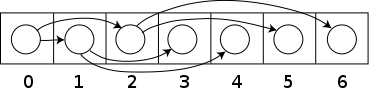
Binary trees can also be stored in breadth-first order as an implicit data structure in arrays, and if the tree is a complete binary tree, this method wastes no space. In this compact arrangement, if a node has an index i, its children are found at indices ${\displaystyle 2i+1}$ (for the left child) and ${\displaystyle 2i+2}$ (for the right), while its parent (if any) is found at index ${\displaystyle \left\lfloor {\frac {i-1}{2}}\right\rfloor }$ (assuming the root has index zero). Alternatively, with a 1-indexed array, the implementation is simplified with children found at ${\displaystyle 2i}$ and ${\displaystyle 2i+1}$, and parent found at ${\displaystyle \lfloor i/2\rfloor }$.^[28] This method benefits from more compact storage and better locality of reference, particularly during a preorder traversal. However, it is expensive to grow^{[citation needed]} and wastes space proportional^{[citation needed]} to 2^h - n for a tree of depth h with n nodes.

This method of storage is often used for binary heaps.^{[citation needed]}

Encodings

Succinct encodings

A succinct data structure is one which occupies close to minimum possible space, as established by information theoretical lower bounds. The number of different binary trees on ${\displaystyle n}$ nodes is ${\displaystyle \mathrm {C} _{n}}$, the ${\displaystyle n}$th Catalan number (assuming we view trees with identical structure as identical). For large ${\displaystyle n}$, this is about ${\displaystyle 4^{n}}$; thus we need at least about ${\displaystyle \log _{2}4^{n}=2n}$ bits to encode it. A succinct binary tree therefore would occupy ${\displaystyle 2n+o(n)}$ bits.

One simple representation which meets this bound is to visit the nodes of the tree in preorder, outputting "1" for an internal node and "0" for a leaf. [1] If the tree contains data, we can simply simultaneously store it in a consecutive array in preorder. This function accomplishes this:

function EncodeSuccinct(node n, bitstring structure, array data) {
    if n = nil then
        append 0 to structure;
    else
        append 1 to structure;
        append n.data to data;
        EncodeSuccinct(n.left, structure, data);
        EncodeSuccinct(n.right, structure, data);
}

The string structure has only ${\displaystyle 2n+1}$ bits in the end, where ${\displaystyle n}$ is the number of (internal) nodes; we don't even have to store its length. To show that no information is lost, we can convert the output back to the original tree like this:

function DecodeSuccinct(bitstring structure, array data) {
    remove first bit of structure and put it in b
    if b = 1 then
        create a new node n
        remove first element of data and put it in n.data
        n.left = DecodeSuccinct(structure, data)
        n.right = DecodeSuccinct(structure, data)
        return n
    else
        return nil
}

More sophisticated succinct representations allow not only compact storage of trees but even useful operations on those trees directly while they're still in their succinct form.

Encoding general trees as binary trees

There is a one-to-one mapping between general ordered trees and binary trees, which in particular is used by Lisp to represent general ordered trees as binary trees. To convert a general ordered tree to a binary tree, we only need to represent the general tree in left-child right-sibling way. The result of this representation will automatically be a binary tree if viewed from a different perspective. Each node N in the ordered tree corresponds to a node N' in the binary tree; the left child of N' is the node corresponding to the first child of N, and the right child of N' is the node corresponding to N 's next sibling --- that is, the next node in order among the children of the parent of N. This binary tree representation of a general order tree is sometimes also referred to as a left-child right-sibling binary tree (also known as LCRS tree, doubly chained tree, filial-heir chain).

One way of thinking about this is that each node's children are in a linked list, chained together with their right fields, and the node only has a pointer to the beginning or head of this list, through its left field.

For example, in the tree on the left, A has the 6 children {B,C,D,E,F,G}. It can be converted into the binary tree on the right.

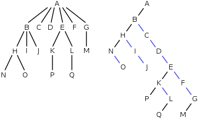
The binary tree can be thought of as the original tree tilted sideways, with the black left edges representing first child and the blue right edges representing next sibling. The leaves of the tree on the left would be written in Lisp as:

(((N O) I J) C D ((P) (Q)) F (M))

which would be implemented in memory as the binary tree on the right, without any letters on those nodes that have a left child.

Common operations

Tree rotations are very common internal operations on self-balancing binary trees.

There are a variety of different operations that can be performed on binary trees. Some are mutator operations, while others simply return useful information about the tree.

Insertion

Nodes can be inserted into binary trees in between two other nodes or added after a leaf node. In binary trees, a node that is inserted is specified as to whose child it will be.

Leaf nodes

To add a new node after leaf node A, A assigns the new node as one of its children and the new node assigns node A as its parent.

Internal nodes

The process of inserting a node into a binary tree

Insertion on internal nodes is slightly more complex than on leaf nodes. Say that the internal node is node A and that node B is the child of A. (If the insertion is to insert a right child, then B is the right child of A, and similarly with a left child insertion.) A assigns its child to the new node and the new node assigns its parent to A. Then the new node assigns its child to B and B assigns its parent as the new node.

Deletion

Deletion is the process whereby a node is removed from the tree. Only certain nodes in a binary tree can be removed unambiguously.^[29]

Node with zero or one children

The process of deleting an internal node in a binary tree

Suppose that the node to delete is node A. If A has no children, deletion is accomplished by setting the child of A's parent to null. If A has one child, set the parent of A's child to A's parent and set the child of A's parent to A's child.

Node with two children

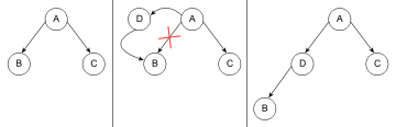
In a binary tree, a node with two children cannot be deleted unambiguously.^[29] However, in certain binary trees (including binary search trees) these nodes can be deleted, though with a rearrangement of the tree structure.

Traversal

Pre-order, in-order, and post-order traversal visit each node in a tree by recursively visiting each node in the left and right subtrees of the root.

Depth-first order

In depth-first order, we always attempt to visit the node farthest from the root node that we can, but with the caveat that it must be a child of a node we have already visited. Unlike a depth-first search on graphs, there is no need to remember all the nodes we have visited, because a tree cannot contain cycles. Pre-order is a special case of this. See depth-first search for more information.

Breadth-first order

Contrasting with depth-first order is breadth-first order, which always attempts to visit the node closest to the root that it has not already visited. See breadth-first search for more information. Also called a level-order traversal.

In a complete binary tree, a node's breadth-index (i − (2^d − 1)) can be used as traversal instructions from the root. Reading bitwise from left to right, starting at bit d − 1, where d is the node's distance from the root (d = ⌊log₂(i+1)⌋) and the node in question is not the root itself (d > 0). When the breadth-index is masked at bit d − 1, the bit values 0 and 1 mean to step either left or right, respectively. The process continues by successively checking the next bit to the right until there are no more. The rightmost bit indicates the final traversal from the desired node's parent to the node itself. There is a time-space trade-off between iterating a complete binary tree this way versus each node having pointer/s to its sibling/s.

See also

References

Citations

Bibliography

• Donald Knuth. The Art of Computer Programming vol 1. Fundamental Algorithms, Third Edition. Addison-Wesley, 1997. ISBN 0-201-89683-4. Section 2.3, especially subsections 2.3.1–2.3.2 (pp. 318–348).

External links

• binary trees entry in the FindStat database
• Binary Tree Proof by Induction
• Balanced binary search tree on array How to create bottom-up an Ahnentafel list, or a balanced binary search tree on array
• Binary trees and Implementation of the same with working code examples
• Binary Tree JavaScript Implementation with source code